What is CTI?

Charge Transfer Inefficiency, or CTI for short, is an effect that occurs when acquiring imaging data from Charge Coupled Devices (CCDs).

Lets take a look at a extract of data taken from the Advanced Camera for Surveys (ACS) instrument on board the Hubble Space Telescope (this figure is taken from Massey et al 2009 https://arxiv.org/abs/1009.4335):

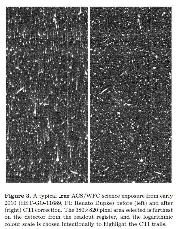
Trailing

On the left hand side of the figure, we can see CTI is action. Upwards from all the bright sources of light (which are of galaxies, stars and cosmic rays) we see a trailing or smearing effect. This is not a genuine signal emitted by each galaxy or star, but is instead induced during data acquisition.

On the right hand side of the figure, we can see that when a CTI correction is applied this trailing effect is entirely removed from the data.

This trailing effect is the characteristic signal of Charge Transfer Inefficiency, and removing it is pretty much what PyAutoCTI is all about!

CCD Clocking

To understand at a physical level what CTI is, we first need to understand how a CCD acquires imaging data. This is a massive over simplification, but in order to understand CTI this process can be simplified into 4 steps:

1. Point a telescope (e.g. the Hubble Space Telescope) towards light sources (e.g. stars, galaxies, etc.) whose photons are collected via the telescope mirror and hit the CCD.

2. These photons interact with a silicon lattice inside the CCD and via the photoelectric effect are converted into (photo-)electrons. These electrons make-up the signal that we observe (e.g. the galaxies, stars and cosmic rays in the image above).

3. Left to their own accord, these electrons would move freely over the CCD and we would lose our image of the galaxies and stars. Therefore, an electrostatic potential runs over the CCD, which applies voltage difference that hold electrons in place wherever they interacted with the silicon lattice. The electrons therefore maintain their 2D spatial locations, corresponding to the 2D pixels we see in the image above.

4. We finally convert this analogue signal of electrons into a digital image. By varying the voltages of the electrostatic potential we can move electrons across the CCD, towards the ‘read-out electronics’ which perform this analogue to digital conversion. The end result of this process is a 2D digital image, like the one shown above.

The animation below shows this process in action:

CTI

Now we know how a CCD works, we can understand what CTI is.

During the CCD clocking process, there are defections and imperfections in the CCD’s silicon lattice, called ‘traps’. These traps capture electrons and hold them for a certain amount of time. Depending on the length of time they hold the electron, one of two things can happen:

• The release time is shorter than the clocking speed of the CCD, such that the electron is released with its original group of electrons that are collectively held together in the same electrostatic potential (e.g. they all correspond to the same pixel in the image). In this case there is no trailing or smearing.

• The release time is longer than the clocking speed of the CCD. In this case, the electron’s original group of electrons have already moved on, well away from the electron. This means that when the electron is released, it joins a different group of electrons in a preceeeding electrostatic potential (e.g. the electrons appears in a different image pixel). Clearly, this is responsible for the trailing effect we’ve seen in the images above!

The animation below shows the CCD clocking process, but now includes one of these traps:

Charge Transfer

We can now understand why CTI is called Charge Transfer Inefficiency: it is simply the inefficient transfer of charge (e.g.a flow of electrons)!

Now, lets quickly show how we can model CTI using PyAutoCTI.

To use PyAutoCTI we first import autocti and the plot module.

import autocti as ac
import autocti.plot as aplt

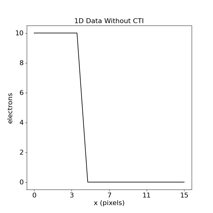
Firstly, lets create a simple 1D dataset, which could correspond to a column of data in a 2D image like those shown above. For simplicity, this data is 5 pixels each containing 100 electrons with 10 empty pixels trailing them.

The Array1D object is a class representing a 1D data structure. It inherits from a numpy ndarray but is extended with functionality which is expanded upon elsewhere in the workspace.

pre_cti_data_1d = ac.Array1D.no_mask(
            values=[10.0, 10.0, 10.0, 10.0, 10.0, 0.0, 0.0, 0.0, 0.0, 0.0, 0.0, 0.0, 0.0, 0.0, 0.0],
    pixel_scales=1.0,
)

PyAutoCTI has a built in visualization library for plotting 1D data (amongst many other things)!

(The aplt.Title() object below wraps the matplotlib method plt.title() – the PyAutoCTI visualization library has numerous wrappers like this which will crop up throughout the overview tutorials).

array_1d_plotter = aplt.Array1DPlotter(y=pre_cti_data_1d)
array_1d_plotter.figure_1d()

arCTIc

To model the CCD clocking process, including CTI, we use arCTIc, or the “algorithm for Charge Transfer Inefficiency clocking”.

arCTIc is written in c++ can be used standalone outside of PyAutoCTI as described on its GitHub page (https://github.com/jkeger/arctic). PyAutoCTI uses arCTIc’s built-in Python wrapper.

In PyAutoCTI we call arCTIc via a Clocker object, which is a Python class that wraps arCTIc. This class has many optional inputs that customize how clocking is performed, but we’ll omit these for now to keep things simple.

clocker_1d = ac.Clocker1D()

CTI Model

We now need to define our CTI model, that is the number of traps our 1D data is going to encounter when we pass it through the clocker and replicate the CCD clocking process..

There are many different types of traps one can use do to this. We will use the simplest, a TrapInstantCapture, which instantaneously captures an electron when it encounters it during CCD clocking.

The number of these traps our 1D data encounters is set via the density parameter, whereas the release_timescale defines how long, on average, each trap holds an electron for (we discuss what units these parameters are in and therefore what they physically mean elsewhere in the workspace).

trap = ac.TrapInstantCapture(density=1.0, release_timescale=5.0)

CTI also depends on the physical properties of the CCD, and how each group of electrons (called a ‘cloud’ of electrons) interacts with the silicon lattice. We’ll describe this in more detail elsewhere, but it does mean we need to also define a CCDPhase class before we can clock our data using arCTIc.

ccd = ac.CCDPhase(well_fill_power=0.58, well_notch_depth=0.0, full_well_depth=200000.0)

We group these into a CTI1D object.

cti = ac.CTI1D(trap_list=[trap], ccd=ccd)

We can now add CTI to our 1D data by passing it through the 1D clocker.

Note that, in 1D, clocking is to the left of the image.

post_cti_data_1d = clocker_1d.add_cti(data=pre_cti_data_1d, cti=cti)

array_1d_plotter = aplt.Array1DPlotter(y=post_cti_data_1d)
array_1d_plotter.figure_1d()

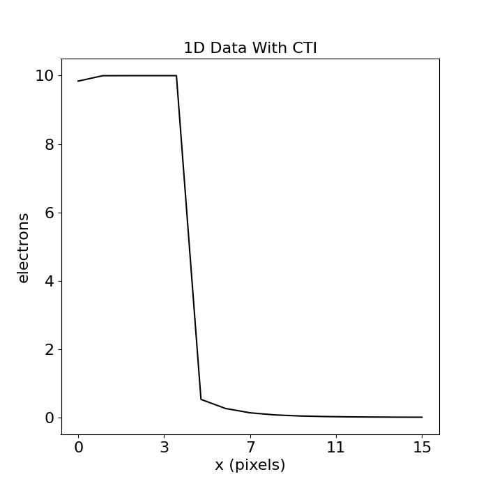
We can see CTI add been added to our 1D data!

To the right of our 5 pixels which each contained 10 electrons, we can now see a faint signal has emerged when previously all that was there were pixels containig 0 electrons. This is CTI trailing; electrons have been trailed from the pixels with 10 electrons into these trailing pixels, as a result of CTI.

We can also see that the pixels which previously contained 100 electrons now have slightly less, they have lost electrons. This makes sense – when electrons are trailed due to CTI they are moved from one pixel i nto another pixel behind it. We therefore should expect that the pixels at the front lose electrons.

Correcting CTI

Using a CTI model and clocker we added CTI to a 1D data, degrading our original signal of 5 pixels containing 10 electrons.

Fortunately, arCTIc can also correct CTI. To do this, we simply pass it the data we want to correct (which therefore ought to include CTI) and the CTI model we will use to correct it. We will use the data with CTI we just created above, alongside the CTI model used to create it.

corrected_cti_data_1d = clocker_1d.remove_cti(data=post_cti_data_1d, cti=cti)

array_1d_plotter = aplt.Array1DPlotter(y=corrected_cti_data_1d)
array_1d_plotter.figure_1d()

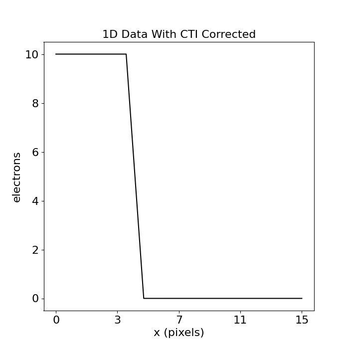
We have corrected CTI from the data and almost recovered our original 1D dataset!

The CTI correction uses an iterative approach, where it uses the add_cti function to add CTI to the input data. Each calls informs arCTIc of how the CTI model relocates (e.g. trails) electrons, which arCTIc then uses to figure out how to moves electrons back to their original pixel.

By iteratively performing this operation muitliple times (typically 5 times) more and more electrons are relocated to their original pixels. Eventually, the CTI trails in the input data are removed and arCTIc no longer moves any electrons after each iteration.

What Forms Traps?

We now understand that CTI is caused by traps in the silicon lattice, but why do these traps exist? How do they form?

A very small number of traps form during CCD manufacturing, we are talking about a tiny amount. Most CCD manufacturing is so good nowadays, that the level of CTI is < 0.000001%. That is, for every electron we move over a pixel, < 0.000001% of transfers lead to an electron being moved into a trailing pixel. This is so small we would probably never even notice CTI in the images, and wouldn’t need to worry about correcting it.

CTI becomes a problem when our telescope is in space. In space, we don’t have the Earth’s atmosphere shielding our telescope from lots of nasty radiation, some of which hits our CCD, interacts with the silicon lattice and forms traps. The longer our telescope has been in space, the more radiation will have hit it, the more traps that will have formed. The figure below slows the level of CTI in Hubble over the course of its lifetime – as a function of time, CTI increases.

Wrap Up

We now have an idea as to what Charge Transfer Inefficiency, or CTI, is. The next overview scripts will expand on the simple toy model we introduced here and add more nuance to the phenomena.

To wrap up, lets consider why we actually care about CTI. Put simply, CTI is a massive problem for many Astronomy science-cases:

• Dark Matter: By measuring the shapes of galaxies to equisite precision a phenomena called ‘weak gravitational lensing’ can be used to map out dark matter throughout the Universe. If our observations of galaxies have this trailing / smearing effect, there is no way we can reliable measure their shapes!

• Exoplanets: Detecting an exoplanet relies on understanding exactly where a small packet of photons hit a CCD, something which a trailing / smearing effect does not make straight forward.