Fitting#
CTI calibration is the process of determining the CTI model of a given CCD, including the total density of traps on the CCD, the average release times of these traps and the CCD filling behaviour.
To perform CTI calibration, we first need to be able to assume a CTI model, fit it to a dataset (e.g. charge injection imaging) and quantify its goodness-of-fit.
If we can do this, we are then in a position to perform CTI calibration via a non-linear fitting algorithm (which is the topic of the next overview). This overview shows how we fit data with a CTI model using PyAutoCTI.
Fitting a CTI model to a realistically sized charge injection image (e.g. the 2066 x 2128 images of previous tutorials) can take a while. To ensure this illustration script runs fast, we’ll fit an idealized charge injection image which is just 30 x 30 pixels.
Dataset (Charge Injection)#
We set up the variables required to load the charge injection imaging, using the same code shown in the previous overview.
Note that the Region2D and Layout2DCI inputs have been updated to reflect the 30 x 30 shape of the dataset.
shape_native = (30, 30)

parallel_overscan = ac.Region2D((25, 30, 1, 29))
serial_prescan = ac.Region2D((0, 30, 0, 1))
serial_overscan = ac.Region2D((0, 25, 29, 30))

regions_list = [(0, 25, serial_prescan[3], serial_overscan[2])]

layout = ac.Layout2DCI(
    shape_2d=shape_native,
    region_list=regions_list,
    parallel_overscan=parallel_overscan,
    serial_prescan=serial_prescan,
    serial_overscan=serial_overscan,
)
We load a charge injection image with injections of 100e-.
normalization = 100

dataset_label = "overview"
dataset_type = "calibrate"
dataset_path = path.join("dataset", "imaging_ci", dataset_label, dataset_type)

dataset = ac.ImagingCI.from_fits(
    data_path=path.join(dataset_path, f"data_{int(normalization)}.fits"),
    noise_map_path=path.join(dataset_path, f"noise_map_{int(normalization)}.fits"),
    pre_cti_data_path=path.join(
        dataset_path, f"pre_cti_data_{int(normalization)}.fits"
    ),
    layout=layout,
    pixel_scales=0.1,
)
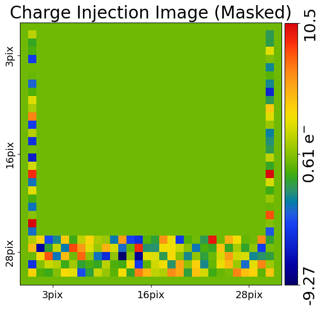
By plotting the charge injection image, we see that it is a 30 x 30 cutout of a charge injection region.
The dataset has been simulated with only parallel CTI, and therefore only contains a single FPR (at the top of each image) and a single EPER (with trails appearing at the bottom of the image).
We will fit only a parallel CTI model for simplicity in this overview, but extending this to also include serial CTI is straightforward.
dataset_plotter = aplt.ImagingCIPlotter(dataset=imaging_ci)
dataset_plotter.figures_2d(data=True, pre_cti_data=True)
CTI Model#
We next illustrate how we fit this charge injection imaging with a parallel CTI model and quantify the goodness of fit.
We therefore need to assume a parallel CTI which we fit to the data.
We therefore set up a clocker, traps and a CCD volume filling phase.
clocker_2d = ac.Clocker2D()

parallel_trap = ac.TrapInstantCapture(density=1.0, release_timescale=2.0)
parallel_ccd = ac.CCDPhase(
    well_fill_power=0.75, well_notch_depth=0.0, full_well_depth=200000.0
)

cti = ac.CTI2D(parallel_trap_list=[parallel_trap], parallel_ccd=parallel_ccd)
Charge Injection Fitting#
To fit the CTI model to our charge injection imaging we create a post_cti_image via the clocker and pass it with
the dataset to the FitImagingCI object.
post_cti_image = clocker_2d.add_cti(
    data=dataset.pre_cti_data,
    cti=cti
)

fit = ac.FitImagingCI(dataset=dataset, post_cti_data=post_cti_image)
From here on, we refer to the post_cti_image as our model_image – it is the image of our CTI model which we are
comparing to the data to determine whether the CTI model is a good fit.
The FitImagingCI object contains both these terms as properties, however they both correspond to the same 2D numpy
array.
print(fit.post_cti_data.native[0, 0])
print(fit.model_image.native[0, 0])
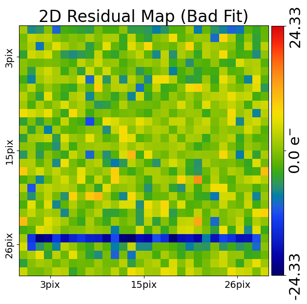
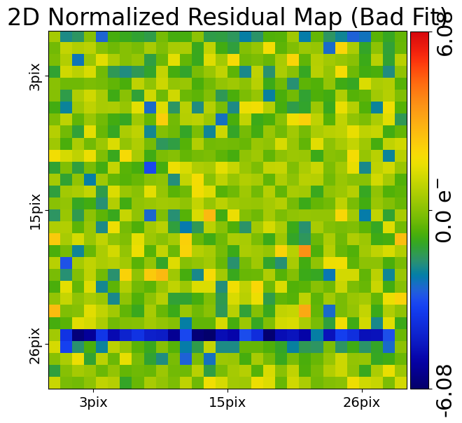
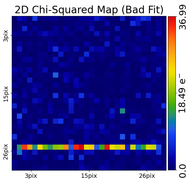
The FitImagingCI contains the following NumPy arrays as properties which quantify the goodness-of-fit:
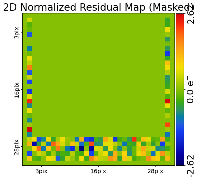
residual_map: Residuals = (Data - Model_Data).
normalized_residual_map:` Normalized_Residual = (Data - Model_Data) / Noise
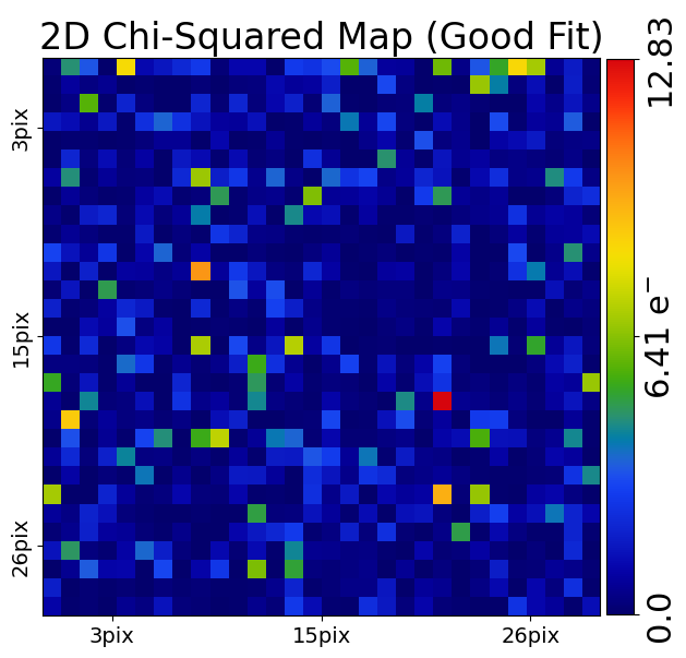
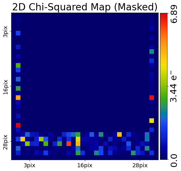
chi_squared_map: Chi_Squared = ((Residuals) / (Noise)) ** 2.0 = ((Data - Model)**2.0)/(Variances)
We can plot these via a FitImagingCIPlotter and see that the residuals and other quantities are significant,
indicating a bad model fit.
fit_plotter = aplt.FitImagingCIPlotter(fit=fit)
fit_plotter.figures_2d(
    residual_map=True, normalized_residual_map=True, chi_squared_map=True
)
There are single valued floats which quantify the goodness of fit:
chi_squared: The sum of thechi_squared_map.
noise_normalizationalization: The normalizing noise term in the likelihood functionwhere [Noise_Term] = sum(log(2*pi*[Noise]**2.0)).
An overall goodness-of-fit measurement is provided by the log_likelihood:
log_likelihood: The log likelihood value of the fit where [LogLikelihood] = -0.5*[Chi_Squared_Term + Noise_Term].
print(fit.chi_squared)
print(fit.noise_normalizationalization)
print(fit.log_likelihood)
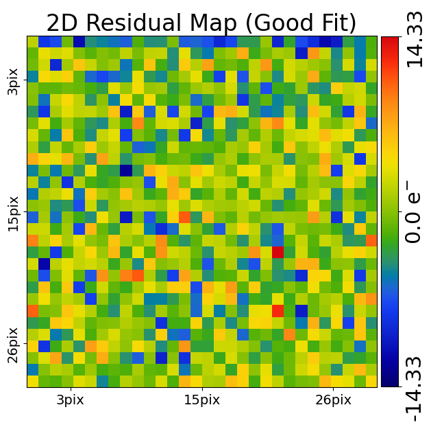
Good Fit#
The significant residuals indicate the model-fit above is bad.
Below, we use the “correct” CTI model (which we know because it is the model we used to simulate this charge injection data!) to reperform the fit above.
parallel_trap_0 = ac.TrapInstantCapture(density=10.0, release_timescale=5.0)
parallel_trap_list = [parallel_trap_0]

parallel_ccd = ac.CCDPhase(
    well_fill_power=0.5, well_notch_depth=0.0, full_well_depth=200000.0
)

post_cti_data = clocker_1d.add_cti(data=dataset.pre_cti_data, cti=cti)

fit = ac.FitImagingCI(dataset=dataset, post_cti_data=post_cti_image)
The plot of the residuals now shows no significant signal, indicating a good fit.
fit_plotter = aplt.FitImagingCIPlotter(fit=fit)
fit_plotter.figures_2d(
    residual_map=True, normalized_residual_map=True, chi_squared_map=True
)
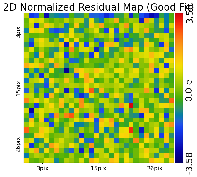
If we compare the log_likelihood to the value above, we can see that it has increased by a lot, again indicating a
good fit.
You should keep the quantity the log_likelihood in mind as it will be key when we discuss how CTI calibration is
performed.
print(fit.log_likelihood)
Masking#
We may want to fit charge injection data but mask regions of the data such that it is not including it the fit.
PyAutoCTI has built in tools for masking. For example, below, we create a mask which removes all 25 pixels containing the parallel FPR.
mask = ac.Mask2D.all_false(
    shape_native=dataset.shape_native, pixel_scales=dataset.pixel_scales
)

mask = ac.Mask2D.masked_fpr_and_eper_from(
    mask=mask,
    layout=dataset.layout,
    pixel_scales=dataset.pixel_scales,
    settings=ac.SettingsMask2D(parallel_fpr_pixels=(0, 25)),
)
If we apply this mask to the charge injection imaging and plot it, the parallel FPR is remove from the plotted figure.
dataset = dataset.apply_mask(mask=mask)

dataset_plotter = aplt.ImagingCIPlotter(dataset=imaging_ci)
dataset_plotter.figures_2d(data=True)
If we repeat the fit above using this masked imaging we see that the residuals, normalized residuals and chi-squared map are masked and not included in the fit.
fit = ac.FitImagingCI(dataset=dataset, post_cti_data=post_cti_image)

fit_plotter = aplt.FitImagingCIPlotter(fit=fit)
fit_plotter.figures_2d(
    residual_map=True, normalized_residual_map=True, chi_squared_map=True
)
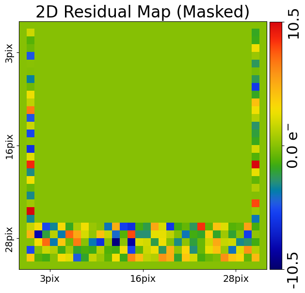
Furthermore, the log_likelihood value changes, because the parallel FPR pixels are not used when computing its value.
print(fit.log_likelihood)
Fitting 1D Datasets#
In previous tutorials, we illustrated CTI using 1D datasets which contained an FPR and EPER.
Below we load a 1D dataset which you can imagine corresponds to a single column of a charge injection image:
shape_native = (30,)

prescan = ac.Region1D((0, 1))
overscan = ac.Region1D((25, 30))

region_list = [(1, 25)]

normalization = 100

layout = ac.Layout1D(
        shape_1d=shape_native,
        region_list=region_list,
        prescan=prescan,
        overscan=overscan,
    )

dataset = ac.Dataset1D.from_fits(
    data_path=path.join(dataset_path, f"data_{int(normalization)}.fits"),
    noise_map_path=path.join(dataset_path, f"noise_map_{int(normalization)}.fits"),
    pre_cti_data_path=path.join(
        dataset_path, f"pre_cti_data_{int(normalization)}.fits"
    ),
    layout=layout,
    pixel_scales=0.1,
)
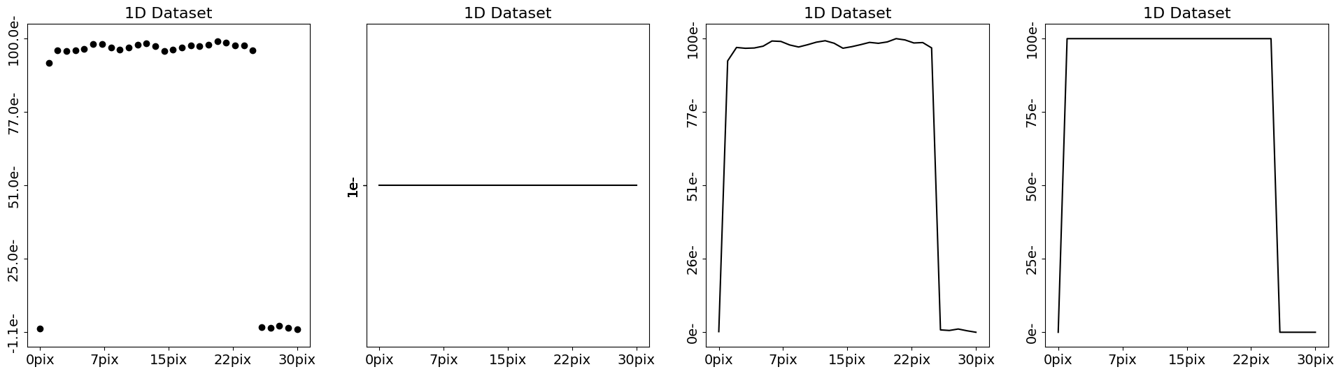
When we plot the dataset we see it has an FPR of 25 pixels and an EPER of 5 trailling pixels, just like the charge injection data.
dataset_plotter = aplt.Dataset1DPlotter(dataset=dataset)
dataset_plotter.subplot_dataset()
We can mask the data to remove the FPR just like we did above.
mask = ac.Mask1D.all_false(
    shape_slim=dataset_1d.shape_slim, pixel_scales=dataset_1d.pixel_scales
)

mask = ac.Mask1D.masked_fpr_and_eper_from(
    mask=mask,
    layout=dataset.layout,
    pixel_scales=dataset.pixel_scales,
    settings=ac.SettingsMask1D(fpr_pixels=(0, 25)),
)
To fit this 1D data we create a 1D clockcer, use this to produce a 1D model image and fit it using a FitDataset1D
object.
Note how visualizing the fit for inspection is a lot easier in 1D than 2D.
clocker_1d = ac.Clocker1D(express=2, roe=ac.ROEChargeInjection())

trap = ac.TrapInstantCapture(density=1.0, release_timescale=2.0)
ccd = ac.CCDPhase(
    well_fill_power=0.75, well_notch_depth=0.0, full_well_depth=200000.0
)

post_cti_data = clocker_1d.add_cti(
    data=dataset.pre_cti_data,
    trap_list=[parallel_trap],
    ccd=parallel_ccd,
)

fit = ac.FitDataset1D(dataset=dataset, post_cti_data=post_cti_data)
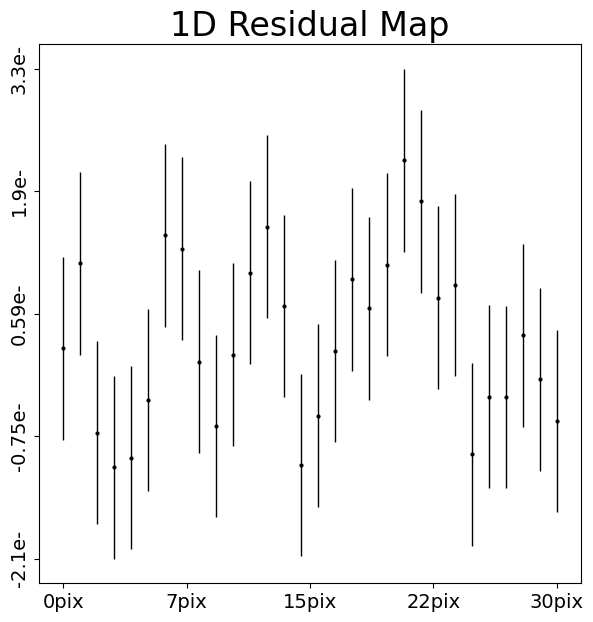
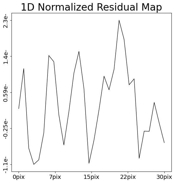
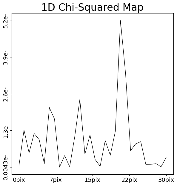
Plotting the fit shows this model gives a good fit, with minimal residuals.
fit_plotter = aplt.FitDataset1DPlotter(fit=fit)
fit_plotter.figures_1d(
    residual_map=True, normalized_residual_map=True, chi_squared_map=True
)
The fit has all the same figures of merit as the charge injection fit, for example, the chi_squared
and log_likelihood.
print(fit.chi_squared)
print(fit.noise_normalizationalization)
print(fit.log_likelihood)
Wrap Up#
This overview shows how by assuming a CTI model, we can use it to create a model-image of a CTI calibration dataset
and fit it to that data. We were able to quantify its goodness-of-fit via a log_likelihood.
We are now in a position to perform CTI calibration, where our goal is to find the CTI model (e.g. the combination
of trap densities, release times and CCD volume filling) which fits the data accurately and gives the highest
log_likelihood values. This is the topic of the next overview.