CTI Calibration#
In the previous overview, we learnt how to fit a CTI model to a dataset and quantify its goodness-of-fit via a log likelihood.
We are now in a position to perform CTI calibration, that is determine the best-fit CTI model to a charge injection dataset. This requires us to perform model-fitting, whereby we use a non-linear search algorithm to fit the model to the data.
CTI modeling uses the probabilistic programming language PyAutoFit, an open-source Python framework that allows complex model fitting techniques to be straightforwardly integrated into scientific modeling software. Check it out if you are interested in developing your own software to perform advanced model-fitting!
Whereas previous tutorials loaded a single charge injection dataset, this tutorial will load and fit three datasets each with a different injection normalizations. This is necessary for us to be able to calibrate the CTI model’s CCD volume filling.
Dataset#
We set up the variables required to load the charge injection imaging, using the same code shown in the previous overview.
Note that the Region2D and Layout2DCI inputs have been updated to reflect the 30 x 30 shape of the dataset.
shape_native = (30, 30)

parallel_overscan = ac.Region2D((25, 30, 1, 29))
serial_prescan = ac.Region2D((0, 30, 0, 1))
serial_overscan = ac.Region2D((0, 25, 29, 30))

regions_list = [(0, 25, serial_prescan[3], serial_overscan[2])]

normalization_list = [100, 1000.0, 10000.0]

total_datasets = len(normalization_list)

layout_list = [
    ac.Layout2DCI(
        shape_2d=shape_native,
        region_list=regions_list,
        parallel_overscan=parallel_overscan,
        serial_prescan=serial_prescan,
        serial_overscan=serial_overscan,
    )
    for i in range(total_datasets)
]
We load each charge injection image, with injections of 100e-, 1000e- and 10000e- so that we have the information required to calibrate the volume filling behaviour of the CCD.
dataset_label = "overview"
dataset_type = "calibrate"
dataset_path = path.join("dataset", "imaging_ci", dataset_label, dataset_type)

imaging_ci_list = [
    ac.ImagingCI.from_fits(
        data_path=path.join(dataset_path, f"data_{int(normalization)}.fits"),
        noise_map_path=path.join(dataset_path, f"noise_map_{int(normalization)}.fits"),
        pre_cti_data_path=path.join(
            dataset_path, f"pre_cti_data_{int(normalization)}.fits"
        ),
        layout=layout,
        pixel_scales=0.1,
    )
    for layout, normalization in zip(layout_list, normalization_list)
]
Clocking#
We define the Clocker which models the CCD read-out, including CTI.
For parallel clocking, we use ‘charge injection mode’ which transfers the charge of every pixel over the full CCD.
clocker = ac.Clocker2D(parallel_express=2, parallel_roe=ac.ROEChargeInjection())
Model#
We compose the CTI model that we fit to the data using autofit Model objects.
These behave analogously to the TrapInstantCapture and CCDPhase objects but their parameters (e.g. density,
well_fill_power) are not specified and are instead determined by a fitting procedure.
In this example we fit a CTI model with:
One parallel
TrapInstantCapture’s which capture electrons during clocking instantly in the parallel direction [2 parameters].A simple
CCDvolume filling parametrization with fixed notch depth and capacity [1 parameter].
The number of free parameters and therefore the dimensionality of non-linear parameter space is N=3.
parallel_trap_0 = af.Model(ac.TrapInstantCapture)
parallel_trap_0.density = af.UniformPrior(lower_limit=0.0, upper_limit=20.0)
parallel_trap_0.release_timescale = af.UniformPrior(lower_limit=0.0, upper_limit=20.0)

parallel_traps = [parallel_trap_0]

parallel_ccd = af.Model(ac.CCDPhase)
parallel_ccd.well_notch_depth = 0.0
parallel_ccd.full_well_depth = 200000.0
We combine the trap and CCD models above into a CTI2D and Collection object, which is the model we will fit.
The CTI2D object can be easily extended to contain model components for serial CTI. Furthermore, the Collection
object can be extended to contain other components of a model other than just the CTI model, for example nuisance
parameters that represent features in the CCD.
model = af.Collection(
    cti=af.Model(ac.CTI2D, parallel_trap_list=[parallel_trap_0], parallel_ccd=parallel_ccd)
)
Printing the info attribute of the model shows us this is the model we are fitting, and shows us the free
parameters and their priors:
print(model.info)
This gives the following output:
cti
    trap_list
        0
            density                              UniformPrior, lower_limit = 0.0, upper_limit = 10.0
            release_timescale                    UniformPrior, lower_limit = 0.0, upper_limit = 50.0
        1
            density                              UniformPrior, lower_limit = 0.0, upper_limit = 10.0
            release_timescale                    UniformPrior, lower_limit = 0.0, upper_limit = 50.0
    ccd
        full_well_depth                          200000.0
        well_notch_depth                         0.0
        well_fill_power                          UniformPrior, lower_limit = 0.0, upper_limit = 1.0
Non-linear Search#
We now choose the non-linear search, which is the fitting method used to determine the set of CTI model parameters that best-fit our data.
In this example we use dynesty (https://github.com/joshspeagle/dynesty), a nested sampling algorithm that is
very effective at lens modeling.
search = af.Nautilus(name="overview_modeling_2d")
Analysis#
analysis_list = [
    ac.AnalysisImagingCI(dataset_ci=imaging_ci, clocker=clocker_2d)
    for dataset in imaging_ci_list
]
By summing this list of analysis objects, we create an overall Analysis which we can use to fit the CTI model, where:
The log likelihood function of this summed analysis class is the sum of the log likelihood functions of each individual analysis object.
The summing process ensures that tasks such as outputting results to hard-disk, visualization, etc use a structure that separates each analysis and therefore each dataset.
analysis = sum(analysis_list)
We can parallelize the likelihood function of these analysis classes, whereby each evaluation is performed on a different CPU.
analysis.n_cores = 1
Model-Fit#
We can now begin the model-fit by passing the model and analysis object to the search, which performs a non-linear search to find which models fit the data with the highest likelihood.
All results are written to hard disk, including on-the-fly results and visualization of the best fit model!
result_list = search.fit(model=model, analysis=analysis)
Result#
The search returns a result object, which includes the charge injection fit corresponding to the maximum log likelihood solution in parameter space for every charge injection dataset.
The info attribute can be printed to give the results in a readable format:
print(result_list.info)
This gives the following output:
Bayesian Evidence                                4125.33026253
Maximum Log Likelihood                           4165.57074867
Maximum Log Posterior                            4165.57074867

model   Collection (N=5)
    cti CTI1D (N=5)
        trap_list                                Collection (N=4)
            0                                    TrapInstantCapture (N=2)
            1                                    TrapInstantCapture (N=2)
        ccd                                      CCDPhase (N=1)

Maximum Log Likelihood Model:

cti
    trap_list
        0
            density                              0.130
            release_timescale                    1.246
        1
            density                              0.251
            release_timescale                    4.401
    ccd
        well_fill_power                          0.580


Summary (3.0 sigma limits):

cti
    trap_list
        0
            density                              0.13 (0.13, 0.13)
            release_timescale                    1.25 (1.23, 1.26)
        1
            density                              0.25 (0.25, 0.25)
            release_timescale                    4.40 (4.37, 4.43)
    ccd
        well_fill_power                          0.58 (0.58, 0.58)


Summary (1.0 sigma limits):

cti
    trap_list
        0
            density                              0.13 (0.13, 0.13)
            release_timescale                    1.25 (1.24, 1.25)
        1
            density                              0.25 (0.25, 0.25)
            release_timescale                    4.40 (4.39, 4.41)
    ccd
        well_fill_power                          0.58 (0.58, 0.58)

instances

cti
    ccd
        full_well_depth                          200000.0
        well_notch_depth                         0.0
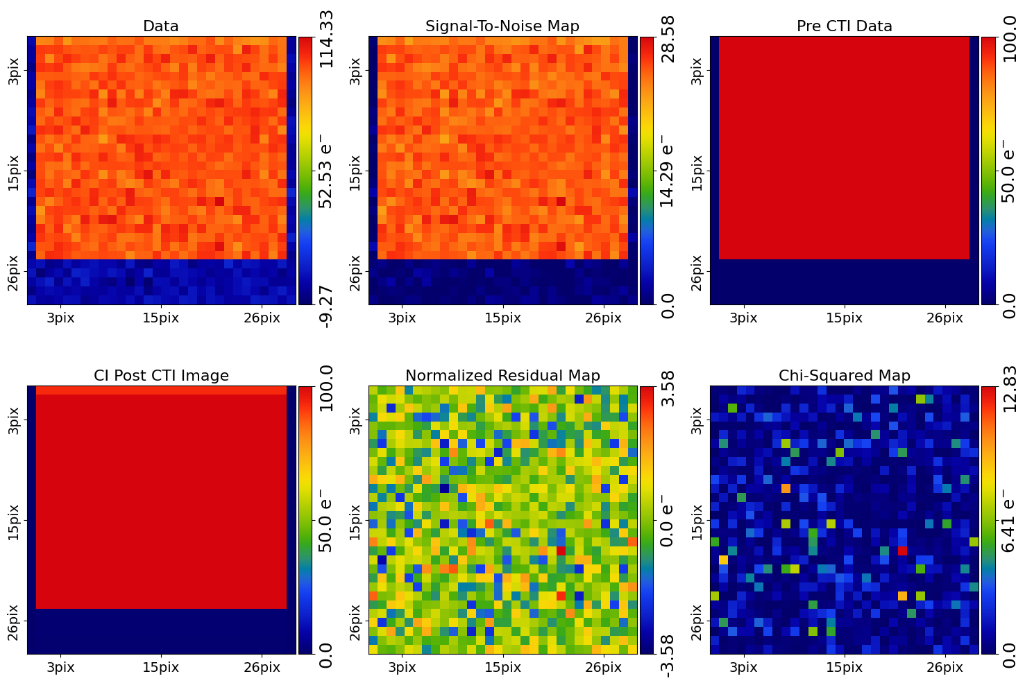
Below, we plot a subplot of the fit for the first dataset which shows a good fit has been inferred.
fit_plotter = aplt.FitImagingCIPlotter(fit=result_list[0].max_log_likelihood_fit)
fit_plotter.subplot_fit()
It also contains the maximum likelihood CTI model, which allows us to print the maximum likelihood values of the inferred CTI model parameters.
Note how this object uses the same API as the Collection and Model we composed above (e.g. the model component
above was named parallel_traps, which is used below).
cti_model = result_list[0].max_log_likelihood_instance.cti

print(cti_model.parallel_traps[0].density)
print(cti_model.parallel_traps[0].release_timescale)
print(cti_model.parallel_ccd.well_fill_power)
Calibration in 1D#
We can also perform CTI calibration on 1D datasets.
shape_native = (30,)

prescan = ac.Region1D((0, 1))
overscan = ac.Region1D((25, 30))

region_list = [(1, 25)]

normalization_list = [100.0, 1000.0, 10000.0]

layout_list = [
    ac.Layout1D(
        shape_1d=shape_native,
        region_list=region_list,
        prescan=prescan,
        overscan=overscan,
    )
    for normalization in normalization_list
]

dataset_list = [
    ac.Dataset1D.from_fits(
        data_path=path.join(dataset_path, f"data_{int(normalization)}.fits"),
        noise_map_path=path.join(dataset_path, f"noise_map_{int(normalization)}.fits"),
        pre_cti_data_path=path.join(
            dataset_path, f"pre_cti_data_{int(normalization)}.fits"
        ),
        layout=layout,
        pixel_scales=0.1,
    )
    for layout, normalization in zip(layout_list, normalization_list)
]

clocker_1d = ac.Clocker1D(express=2)
We define the Clocker1D, which models the CCD read-out, including CTI.
For parallel clocking, we use ‘charge injection mode’ read-out electronics object. Which transfers the charge of every pixel over the full CCD.
clocker_1d = ac.Clocker1D(express=2, roe=ac.ROEChargeInjection())
We again compose a CTI model that we fit to the data using autofit Model objects.
trap_0 = af.Model(ac.TrapInstantCapture)
trap_0.density = af.UniformPrior(lower_limit=0.0, upper_limit=20.0)
trap_0.release_timescale = af.UniformPrior(lower_limit=0.0, upper_limit=50.0)

traps = [trap_0]

ccd = af.Model(ac.CCDPhase)
ccd.well_notch_depth = 0.0
ccd.full_well_depth = 200000.0
We combine the trap and CCD models above into a CTI1D and Collection object, which is the model we will fit.
model = af.Collection(cti=af.Model(ac.CTI1D, traps=traps, ccd=ccd))
We again use dynesty (https://github.com/joshspeagle/dynesty) to fit the model.
search = af.Nautilus(name="overview_modeling_1d")
We next create a list of AnalysisDataset1D objects, which each contain a log_likelihood_function that the
non-linear search calls to fit the CIT model to the data.
We again sum these analyses objects into a single analysis.
analysis_list = [
    ac.AnalysisDataset1D(dataset_1d=dataset_1d, clocker=clocker_1d)
    for dataset in dataset_list
]

analysis = sum(analysis_list)

analysis.n_cores = 1
We can now begin the model-fit by passing the model and analysis object to the search, which performs a non-linear search to find which models fit the data with the highest likelihood.
result_list = search.fit(model=model, analysis=analysis)
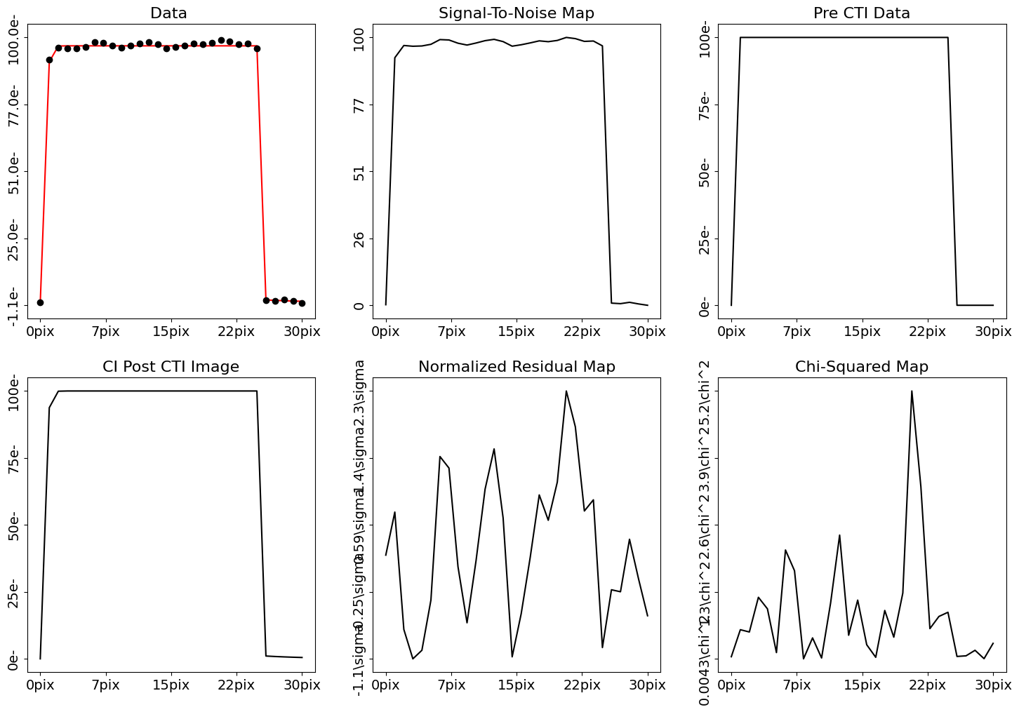
The search returns a result object, which again allows us to print the maximum likelihood CTI model and plot the maximum likelihood fit.
cti_model = result_list[0].max_log_likelihood_instance.cti

print(cti_model.parallel_traps[0].density)
print(cti_model.parallel_traps[0].release_timescale)
print(cti_model.parallel_ccd.well_fill_power)

fit_plotter = aplt.FitDataset1DPlotter(fit=result.max_log_likelihood_fit)
fit_plotter.subplot_fit()
Wrap Up#
A full overview of the CTI results is given at autocti_workspace/*/results.