CTI Features#
To illustrate PyAutoCTI we have assumed different CTI models, which allowed us to add and correct CTI from 1D and 2D data. This model included the properties of the traps on CCD’s silicon lattice and described how electron clouds filled up pixels.
In order to correct CTI in real data, we clearly need this CTI model. But how do we determine it? How do we know how many traps are on a CCD? Or how electrons fill pixels?
To do this, we need to perform CTI calibration, which calibrates our CTI model. In this overview, we’ll take a closer look at charge injection imaging data, and consider why it makes it possible for us to calibrate a CTI model.
To begin, we’ll think about CTI calibration in 1D, before extending this to 2D.
Lets recreate our simple 1D dataset.
import autocti as ac

pre_cti_data_1d = ac.Array1D.no_mask(
            values=[10.0, 10.0, 10.0, 10.0, 10.0, 0.0, 0.0, 0.0, 0.0, 0.0, 0.0, 0.0, 0.0, 0.0, 0.0],
    pixel_scales=1.0,
)
Density Estimate#
We are now going to add CTI to this data using two CTI models, where the trap density of the second model is double that of the first model.
clocker_1d = ac.Clocker1D()

ccd = ac.CCDPhase(well_fill_power=0.58, well_notch_depth=0.0, full_well_depth=200000.0)

trap_0 = ac.TrapInstantCapture(density=250.0, release_timescale=5.0)
trap_1 = ac.TrapInstantCapture(density=500.0, release_timescale=5.0)

cti = ac.CTI1D(trap_list=[trap_0], ccd=ccd)

post_cti_data_1d_0 = clocker_1d.add_cti(data=pre_cti_data_1d, cti=cti)

cti = ac.CTI1D(trap_list=[trap_1], ccd=ccd)

post_cti_data_1d_1 = clocker_1d.add_cti(data=pre_cti_data_1d, cti=cti)
Now lets plot the two datasets and compare their appearance.
array_1d_plotter = aplt.Array1DPlotter(y=post_cti_data_1d_0)
array_1d_plotter.figure_1d()

array_1d_plotter = aplt.Array1DPlotter(y=post_cti_data_1d_1)
array_1d_plotter.figure_1d()
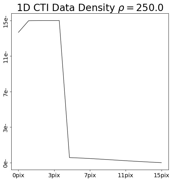

Upon inspection and comparison of each post-CTI dataset, we can note two differences between how CTI has been added.
We are going to term these the First-Pixel Response (FPR) and Extended-Pixel Edge Response (EPER), because these
are the names of each effect in the CTI literature:
First-Pixel Response (FPR): The 5 pixels in the dataset which originally contained 10.0 electrons have different numbers of electrons after CTI is added. The CTI model with a higher density of traps has removed more electrons from these pixels.
Therefore, the region that originally contained a known input number of electrons before CTI is added informs us of how many traps are on the CCD. If the density of traps is higher, the FPR loses more electrons.
Extended-Pixel Edge Response (EPER): The 10 pixels trailing the 5 FPR pixels now have electrons, due to CTI trailing. The CTI model with a higher density has more electrons in the EPER, because it has more traps which capture electrons from the FPR and trail them into the EPER.
Therefore, the region that originally contained no electrons also informs us of how many traps are on the CCD. If the density of traps is higher, the EPER gains more electrons.
By simply summing up how many electrons are moved from the FPR into the EPER one can make a pretty accurate estimate
of the density of traps per pixel (which is the units of density input into the TrapInstantCapture objects above).
Of course, PyAutoCTI actually measures this quantity in a more rigorous way, but we nevertheless have a sense of how to estimate the density of traps on a CCD.
Release Time Estimate#
We now again add CTI to the pre-CTI data using two CTI models, but instead using the same density for each and
increasing the release_timescale of the second CTI model.
clocker_1d = ac.Clocker1D()

ccd = ac.CCDPhase(well_fill_power=0.58, well_notch_depth=0.0, full_well_depth=200000.0)

trap_0 = ac.TrapInstantCapture(density=250.0, release_timescale=0.5)
trap_1 = ac.TrapInstantCapture(density=250.0, release_timescale=3.0)

cti = ac.CTI1D(trap_list=[trap_0], ccd=ccd)

post_cti_data_1d_0 = clocker_1d.add_cti(data=pre_cti_data_1d, cti=cti)

cti = ac.CTI1D(trap_list=[trap_1], ccd=ccd)

post_cti_data_1d_1 = clocker_1d.add_cti(data=pre_cti_data_1d, cti=cti)
Now lets plot the two datasets and compare their appearance.
array_1d_plotter = aplt.Array1DPlotter(y=post_cti_data_1d_0)
array_1d_plotter.figure_1d()

array_1d_plotter = aplt.Array1DPlotter(y=post_cti_data_1d_1)
array_1d_plotter.figure_1d()
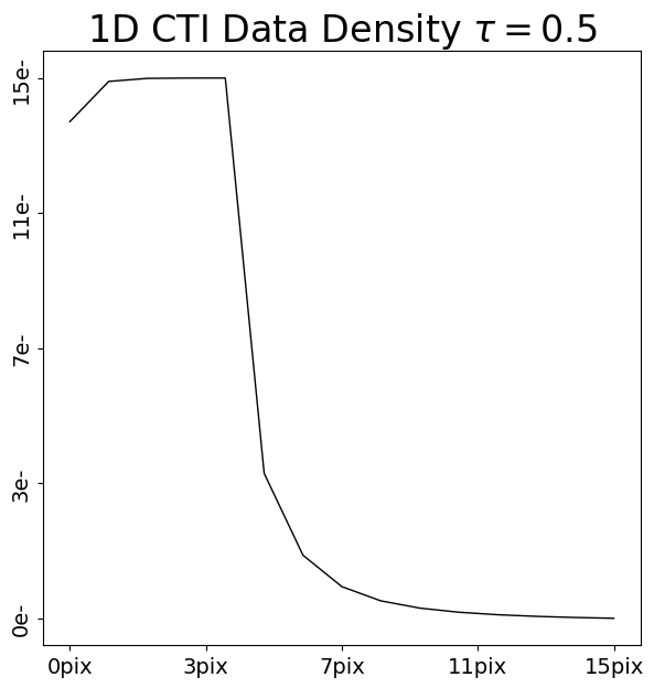
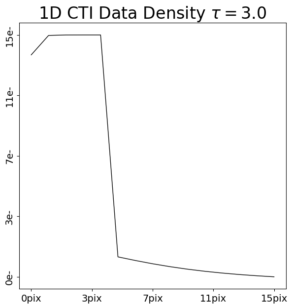
Lets now again compare the FPR and EPER of these two post-CTI datasets:
FPR: Although there are small differences, it is difficult to discern anything obvious. This is because both CTI models have the same density, and therefore the same number of electrons are captured and removed from the FPR.
EPER: The trails in the EPER of the two datasets are clearly different, with the CTI model which used the longer release time ofrelease_timescale=10.0producing a longer trail of electrons. The area under both trails are the same (because the same number of electrons are captured from the FPR and trailed into the EPER), but their shapes are different.
Therefore, the EPER informs us about the release times of the traps in our CTI model.
From solid-state physics, we actually know a lot more about how traps release electrons. The trails observed in each EPER look suspiciously like a 1D exponential, because they are! Traps release electrons according to an exponential probability distribution:
$1 − exp(− (1/τ)$
Where τ is the release_timescale. If a trap has a longer release time, it (on average) releases more electrons over a
wider range of pixels.
CCD Filling#
We now understand how the FPR and EPER of a 1D dataset can inform us on the density of traps in our data, alongside
how they release electrons. But how do we calibrate the CCD volumne filling? The parameters well_fill_power,
well_notch_depth and full_well_depth in the CCDPhase?
The well_notch_depth and full_well_depth are quantities we know about a CCD from its manufacturing process. We
therefore do not need to measure them, we can simply input their values into PyAutoCTI.
The well_fill_power is less straight forward – but what even is it?
In order to describe how a cloud of electrons arCTIc assumes a volume-filling express, for example:
n_c(n_e)=density* ((n_e-full_well_depth) (well_notch_depth-full_well_depth)) **well_fill_beta
Where:
n_e: the number of electrons in a pixel.
n_c: The number of electrons which are captured in that pixel (which depends also on the density of traps).
The key thing to take from this equation is that the number of electrons that are captured depends on both: (i) the
number of electrons in the pixel and; (ii) the well filling parameter well_fill_beta.
Their dependence is non-linear, and depending on the value of well_fill_beta this equation could mean that for fixed
density:
A pixel with 10 electrons in total (
n_e=10) has 2 electrons captured (n_c=2), a 20% capture rate.The same pixel could have contain 100 electrons (
n_e=100) but instead have only 5 electrons captured (n_c=5), a 5% capture rate.
This behaviour is why CTI is such a challenging phenomenon to calibrate and correct.
The way that electrons are captured and release depends non-linearly on the image that is read out.
In order to calibrate this volume filling, we need multiple datasets where the overall normalization of electrons in
each data varies. This samples the volume filling beaviour of the CCD as a function of n_e and thus allow us to
calibrate the well_fill_power.
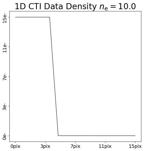
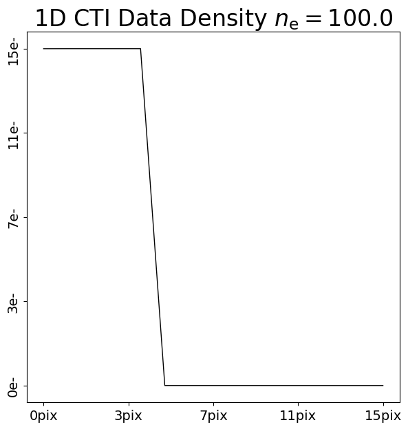
We can illustrate this by comparing the addition of CTI to two 1D datasets with 10 electrons and 100 electrons:
pre_cti_data_1d_0 = ac.Array1D.no_mask(
            values=[10.0, 10.0, 10.0, 10.0, 10.0, 0.0, 0.0, 0.0, 0.0, 0.0, 0.0, 0.0, 0.0, 0.0, 0.0],
    pixel_scales=1.0,
)

pre_cti_data_1d_1 = ac.Array1D.no_mask(
            values=[100.0, 100.0, 100.0, 100.0, 100.0, 0.0, 0.0, 0.0, 0.0, 0.0, 0.0, 0.0, 0.0, 0.0, 0.0],
    pixel_scales=1.0,
)

post_cti_data_1d_0 = clocker_1d.add_cti(data=pre_cti_data_1d_0, cti=cti)
post_cti_data_1d_1 = clocker_1d.add_cti(data=pre_cti_data_1d_1, cti=cti)

array_1d_plotter = aplt.Array1DPlotter(y=post_cti_data_1d_0)
array_1d_plotter.figure_1d()

array_1d_plotter = aplt.Array1DPlotter(y=post_cti_data_1d_1)
array_1d_plotter.figure_1d()