Charge Injection Data#
In overview 2, we inspected charge injection data to understand how 2D CCD clocking works.
Now we know how CTI information is contained in the First-Pixel Response (FPR) and Extended-Pixel Edge Response (EPER) of a dataset, lets consider how a charge injection dataset contains everything we need to calibrate a CTI model.
Lets again load our 2D schematic of a charge injection image:
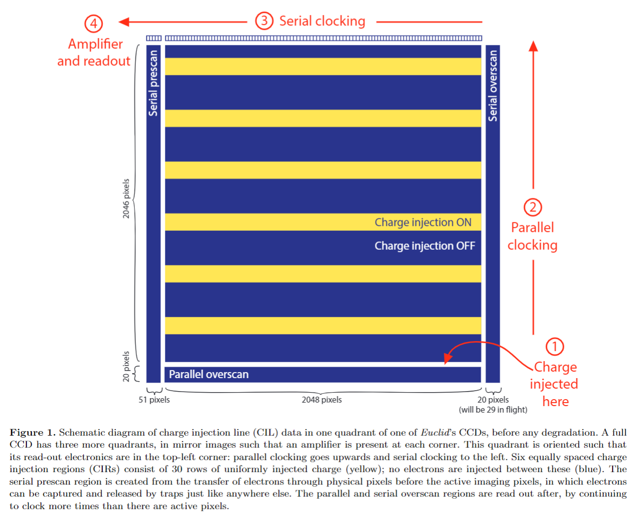
The charge injection electronics create the 2D regions on the data which contain a known input signal of electrons. This is analogous to block of ~10 electrons in our 1D datasets of the previous overviews.
When we acquire a charge injection image using a real CCD, these electrons are subject to CTI. Therefore, a charge injection dataset has FPR’s and EPER’s, just like the 1D dataset we saw in the previous overview. In fact, it has two sets of FPRs and EPERs, corresponding to parallel and serial CTI.
To illustrate this, we will load a charge injection dataset into PyAutoCTI, which has the same dimensions and layout as the schematic above.
Before loading the data we must to define various properties of our charge injection image.
Lets begin by defining the 2D shape_native of our charge injection image, which as discussed in overview 2
has 2046 + 20 = 2066 rows of pixels and 51 + 2048 + 29 = 2128 columns of pixels.
shape_native = (2066, 2128)
Next, we define the regions on the data containing the parallel overscan, serial prescan and serial overscan.
We use a Region2D, which defines a 2D region on the 2D data where the input tuple gives the (y0, y1, x0, x1)
coordinates.
For example, as shown on the schematic, the parallel overscan is at the bottom of the image and its region spans
the pixel coordinates y0 -> y1 = 2108 -> 2128 and x0 -> x1 = 51 -> 2099.
parallel_overscan = ac.Region2D((2108, 2128, 51, 2099))
serial_prescan = ac.Region2D((0, 2128, 0, 51))
serial_overscan = ac.Region2D((0, 2128, 2099, 2128))
We also need to specify the 2D region of every charge injection region (e.g. the pixel coordinates where the charge is injected).
regions_list = [
    (100, 300, serial_prescan[3], serial_overscan[2]),
    (500, 700, serial_prescan[3], serial_overscan[2]),
    (900, 1100, serial_prescan[3], serial_overscan[2]),
    (1300, 1500, serial_prescan[3], serial_overscan[2]),
    (1700, 1900, serial_prescan[3], serial_overscan[2]),
]
We also require the normalization of the injected charge level of each charge injection image in our charge injection imaging dataset.
In this example, we will only inspect one charge injection image with a normalization of 100 electrons.
normalization = 100
We now create a charge injection Layout2DCI object which uses the above variables to describe the different regions
on a charge injection image.
layout = ac.Layout2DCI(
    shape_2d=shape_native,
    region_list=regions_list,
    parallel_overscan=parallel_overscan,
    serial_prescan=serial_prescan,
    serial_overscan=serial_overscan,
)
Now we have defined our layout, we can load the charge injection imaging data as an ImagingCI object.
We have a prepared dataset in the dataset/imaging_ci/overview folder of the workspace which we load below.
The ImagingCI object has the following three attributes:
image: the charge injection image which includes FPRs and EPERs due to CTI.
noise_map: the noise-map of the charge injection image, which below only consists of read noise of 1 electron.
pre_cti_data: an image which estimates what the charge injection image looked like before clocking and therefore without CTI.
dataset_label = "overview"
dataset_type = "uniform"
dataset_path = path.join("dataset", "imaging_ci", dataset_label, dataset_type)

dataset = ac.ImagingCI.from_fits(
    data_path=path.join(dataset_path, f"data_{int(normalization)}.fits"),
    noise_map_path=path.join(dataset_path, f"noise_map_{int(normalization)}.fits"),
    pre_cti_data_path=path.join(
        dataset_path, f"pre_cti_data_{int(normalization)}.fits"
    ),
    layout=layout,
    pixel_scales=0.1,
)
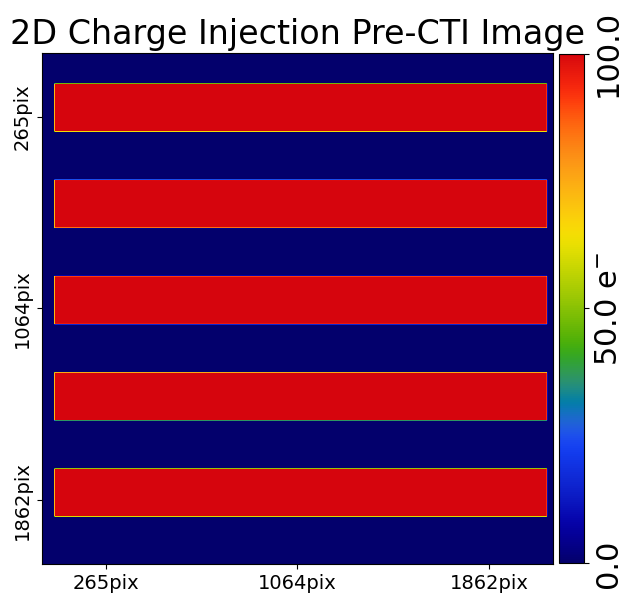
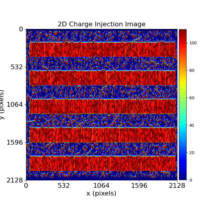
We can plot the charge injection imaging using a ImagingCI object.
dataset_plotter = aplt.ImagingCIPlotter(dataset=imaging_ci)
dataset_plotter.figures_2d(data=True)
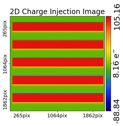
The figure shows the charge injection regions as rectangular blocks interspersed with regions of zero change, as expected.
Furthermore, by closely inspecting the edges of each charge injection plots changes in signal can be seen, corresponding to the parallel and serial FPRs and EPERs.
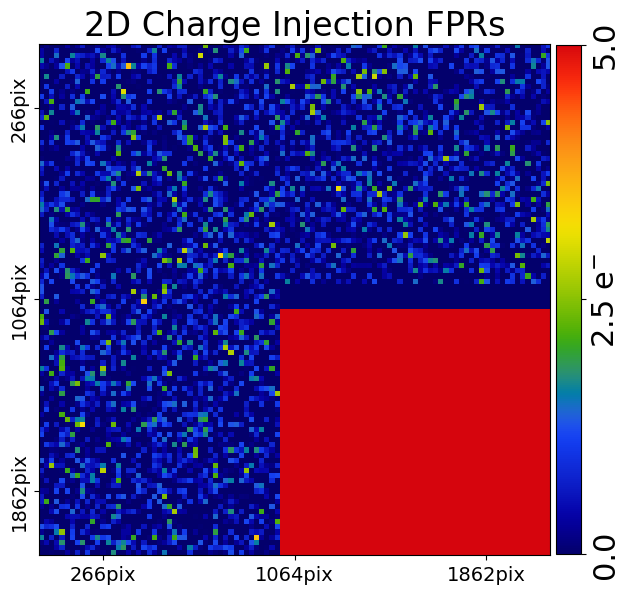
We can zoom in on one of these regions and change the color scheme to properly highlight the FPRs.
(PyAutoCTI has a built-in visualization library which wraps matplotlib, which is documented in the
autocti_workspace/*/plots package).
mat_plot_2d = aplt.MatPlot2D(
    axis=aplt.Axis(extent=[-106.0, -96.0, 88.0, 98.0]),
    cmap=aplt.Cmap(vmin=0.0, vmax=100.0),
)

dataset_plotter = aplt.ImagingCIPlotter(dataset=imaging_ci, mat_plot_2d=mat_plot_2d)
dataset_plotter.figures_2d(data=True)
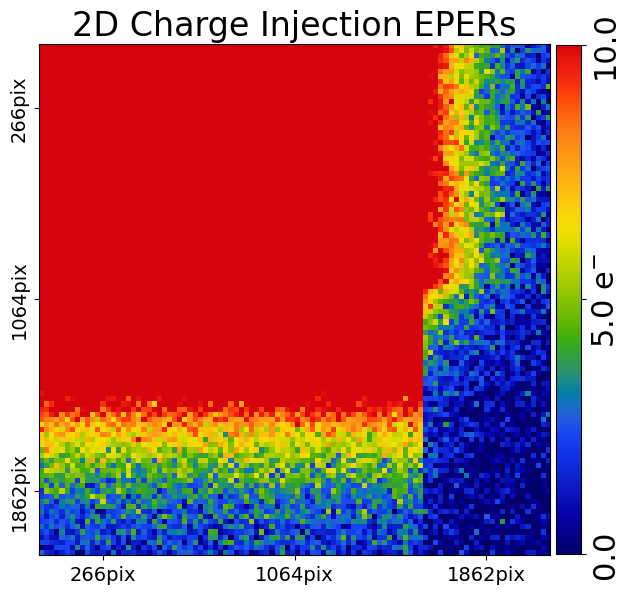
We can do the same to highlight the EPERs.
mat_plot_2d = aplt.MatPlot2D(
    axis=aplt.Axis(extent=[96.0, 106.0, 68.0, 78.0]),
    cmap=aplt.Cmap(vmin=0.0, vmax=10.0),
)

dataset_plotter = aplt.ImagingCIPlotter(dataset=imaging_ci, mat_plot_2d=mat_plot_2d)
dataset_plotter.figures_2d(data=True)
The LayoutCI object we defined above is contained in the ImagingCI object.
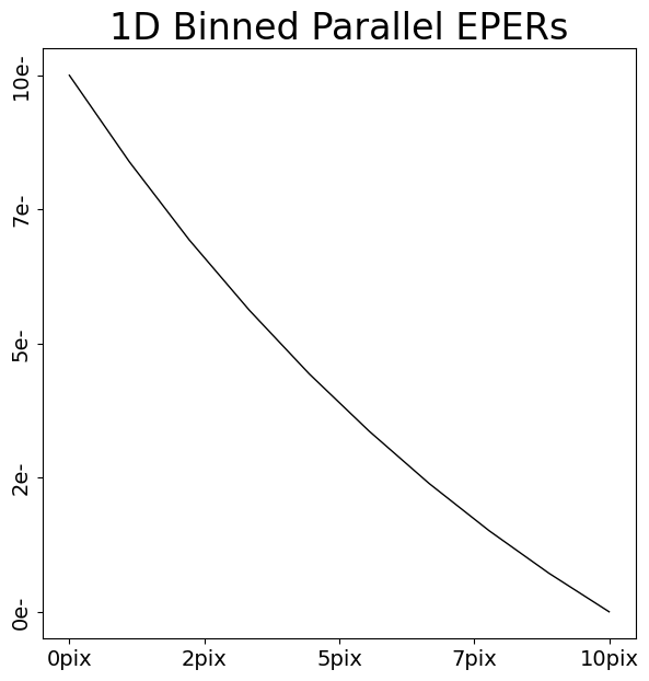
The layout allows us to extract regions of interest in the data, for example a 1D array of the first 10 pixels of every parallel EPERs binned together.
parallel_eper_1d = layout.extract.parallel_eper.binned_array_1d_from(
    array=dataset.data, pixels=(0, 10)
)

array_1d_plotter = aplt.Array1DPlotter(y=parallel_eper_1d)
array_1d_plotter.figure_1d()
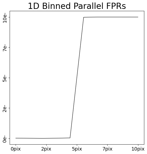
The layout can extract all the regions of interest of the data.
parallel_fpr_1d = layout.extract.parallel_fpr.binned_array_1d_from(
    array=dataset.data, pixels=(0, 10)
)
array_1d_plotter = aplt.Array1DPlotter(y=parallel_fpr_1d)
array_1d_plotter.figure_1d()

serial_eper_1d = layout.extract.serial_eper.binned_array_1d_from(
    array=dataset.data, pixels=(0, 10)
)
array_1d_plotter = aplt.Array1DPlotter(y=serial_eper_1d)
array_1d_plotter.figure_1d()

serial_fpr_1d = layout.extract.serial_fpr.binned_array_1d_from(
    array=dataset.data, pixels=(0, 10)
)
array_1d_plotter = aplt.Array1DPlotter(y=serial_fpr_1d)
array_1d_plotter.figure_1d()

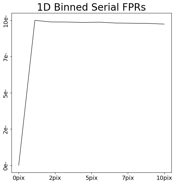
We can now appreciate that charge injection imaging has all the information we need to calibrate CTI – distinct FPR and EPERs.
The other key piece of information is an understanding of what the data looked like before clocking and CTI, which is
contained in the pre_cti_data.
dataset_plotter = aplt.ImagingCIPlotter(dataset=imaging_ci, mat_plot_2d=mat_plot_2d)
dataset_plotter.figures_2d(pre_cti_data=True)
Realistic Charge Injection Imaging#
For the simple charge injection data above this is literally a rectangular of non-zero values (corresponding to the injection level) surrounding large regions of 0 electrons.
The key point is that because when the data was acquired on a CCD, we know what level of charge we injected, we therefore have a clear understanding of its appearance before CTI. Without this knowledge, we could not use it to calibrate CTI.
More realistic charge injection imaging has many other features, for example:
The charge injection may show non-uniformity across the columns. This is not a for CTI calibration provided we have knowledge about the non-uniformity’s appearance during charge injection.
There may be cosmic rays which hit the CCD during data acquisition and are read-out in the data. This is not a problem for CTI calibration provided we can detect, flag and mask these cosmic rays.
PyAutoCTI has built in tools for both these tasks which are illustrated at ?.
dataset_label = "overview"
dataset_type = "non_uniform_cosmic_rays"
dataset_path = path.join("dataset", "imaging_ci", dataset_label, dataset_type)

dataset = ac.ImagingCI.from_fits(
    data_path=path.join(dataset_path, f"data_{int(normalization)}.fits"),
    noise_map_path=path.join(dataset_path, f"noise_map_{int(normalization)}.fits"),
    pre_cti_data_path=path.join(
        dataset_path, f"pre_cti_data_{int(normalization)}.fits"
    ),
    layout=layout,
    pixel_scales=0.1,
)

dataset_plotter = aplt.ImagingCIPlotter(dataset=imaging_ci)
dataset_plotter.figures_2d(data=True, pre_cti_data=True)
Wrap Up#
We now have an understanding of how a dataset, in this case charge injection imaging, can contain the information we need to calibrate a CTI model. We also showed PyAutoCTI’s tools that make loading, manipulating and plotting these datasets straight forward.
Next, we’ll show how we actually compose a CTI model and fit it to a charge injection dataset.