Parallel and Serial#
The descriptions and animations of the previous overview described CCD clocking as a 1D process, whereby electrons were trailed as they move in one direction towards read-out electronics.
However, the images from the Hubble Space Telescope we looked at are 2D, and CCD clocking is of course a 2D process. So, lets adjust our picture of how CCD clocking works to one that is two dimensional.
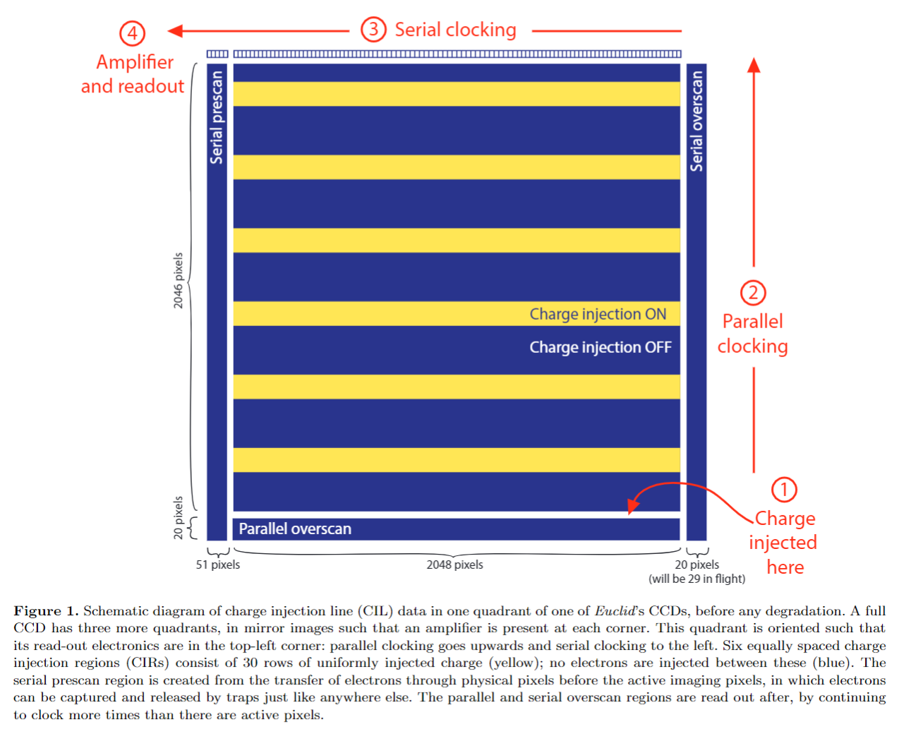
Below is a schematic of a 2D image, called a “charge injection image”. This image does not contain galaxies or stars. Instead, the signal is created using electronics at bottom of the CCD (furthest from the read out electronics) which inject a current (e.g. rows of electrons into every pixel) across the CCD.
This injection is turned on and off, creating the regions of the data with signal (the yellow / orange rectangles in the image below) interspersed around regions with no charge.
(It turns out that charge injection images are crucial to calibrating CTI – a process we have to undertake before we can correct CTI in data. We cover this in overviews 4 and 5!).
Two Dimensional CCD#
The CCD above has 2046 + 20 = 2066 rows of pixels and 51 + 2048 + 29 = 2128 columns of pixels (these are the
dimensions of a CCD quadrant of the Euclid space satellite).
As a reminder, a ‘pixel’ describes a group of electrons that are collectively held together in the same electrostatic potential in the CCD, and therefore read out together in the same pixel after clocking.
Clocking and read-out of a 2D image extends the 1D description above as follows:
An entire row of electrons over 2066 pixels are shifted, all at once, by adjusting the electrostatic potential in every pixel simultaneously. In the diagram above this shift is in the upwards direction.
These electrons enter the special row of pixels shown at the top of the schematic, called the ‘read-out register’, where they are held in place with a special row of electrostatic potentials. This is called ‘parallel clocking’.
At the far end of the read-out register are the read-out electronics. This was seen in the 1D animations in the previous overview and is located at the top-left of the schematic above. The electrons in this row of 2066 pixels, read-out register, are clocked towards read out electronics and converted from an analogue to digital signal. This is called ‘serial clocking.
After the electrons in these 2066 pixels are read out, the read-out register is now empty and the next row of electrons are shifted into it.
This process is repeated until the electrons in all 2128 columns of pixels have been read-out and converted to a digital signal.
In the example above, serial clocking has to shift electrons over 2066 pixels, one pixel at a time, into the read out electronics. For every 2066 shifts, parallel clocking has to move only a single row of electrons (all at once) into the read out register.
Serial clocking is therefore much faster than parallel clocking, in the example above around ~2000 times faster. Keep this in mind!
arCTIc#
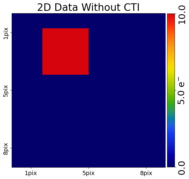
Now, lets perform 2D clocking and CTI addition using arCTIc. First, lets make a scaled down version of the charge injection image, which will simply contain a 3x3 square of pixels containing 100 electrons surrounded by pixels which are empty.
This uses an Array2D object, which is a class representing a 2D data structure and is a 2D extension of the
Array1D objected used in the previous overview. It again inherits from a numpy ndarray and is extended
with functionality which is expanded upon elsewhere in the workspace.
import autocti as ac

pre_cti_data_2d = ac.Array2D.no_mask(
            values=[
        [0.0, 0.0, 0.0, 0.0, 0.0, 0.0, 0.0, 0.0],
        [0.0, 10.0, 10.0, 10.0, 0.0, 0.0, 0.0, 0.0],
        [0.0, 10.0, 10.0, 10.0, 0.0, 0.0, 0.0, 0.0],
        [0.0, 10.0, 10.0, 10.0, 0.0, 0.0, 0.0, 0.0],
        [0.0, 0.0, 0.0, 0.0, 0.0, 0.0, 0.0, 0.0],
        [0.0, 0.0, 0.0, 0.0, 0.0, 0.0, 0.0, 0.0],
        [0.0, 0.0, 0.0, 0.0, 0.0, 0.0, 0.0, 0.0],
        [0.0, 0.0, 0.0, 0.0, 0.0, 0.0, 0.0, 0.0],
        [0.0, 0.0, 0.0, 0.0, 0.0, 0.0, 0.0, 0.0],
        [0.0, 0.0, 0.0, 0.0, 0.0, 0.0, 0.0, 0.0],
    ],
    pixel_scales=0.1,
)
PyAutoCTI has a built in visualization library for plotting 2D data (amongst many other things)!
import autocti.plot as aplt

array_2d_plotter = aplt.Array2DPlotter(array=pre_cti_data_2d)
array_2d_plotter.figure_2d()
To model the CCD clocking process, including CTI, we create a PyAutoCTI Clocker2D object, which calls arCTIc
via a Python wrapper.
clocker_2d = ac.Clocker2D()
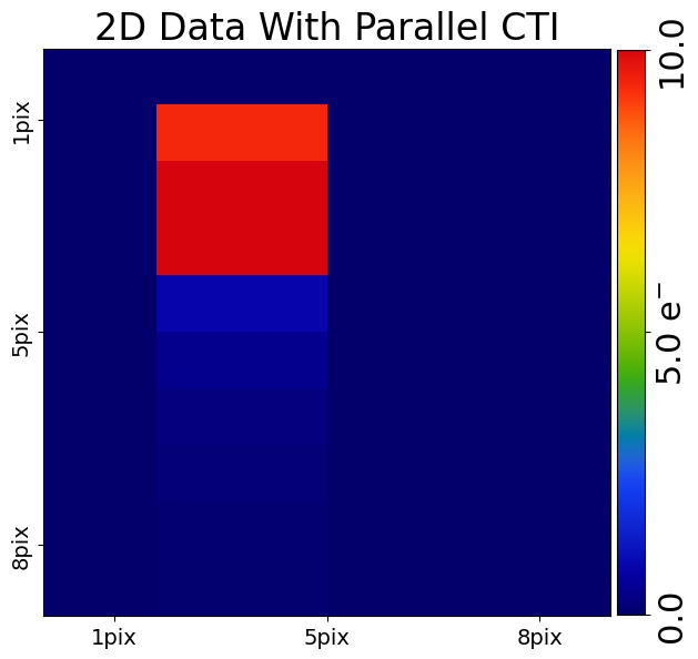
CTI Model (Parallel)#
We again need to define our CTI model, that is the number of traps our 2D data encounters when we pass it through the clocker and replicate the CCD clocking process.
We will again use a trap which captures electrons instantaneously and define the CCD’s phase describing how the electron cloud fills pixels.
You’ll note that the variables below use the prefix parallel_, which indicates that this is only accounting for
CTI in the parallel clocking direction.
parallel_trap = ac.TrapInstantCapture(density=1.0, release_timescale=5.0)
parallel_ccd = ac.CCDPhase(
    well_fill_power=0.58, well_notch_depth=0.0, full_well_depth=200000.0
)
We group these into a CTI2D object.
cti = ac.CTI2D(parallel_trap_list=[parallel_trap], parallel_ccd=parallel_ccd)
We can now add parallel CTI to our 2D data by passing it through the 2D clocker.
For our 2d ndarray which has shape (10,8) parallel clocking goes upwards towards entries in the
row pre_cti_data_2d[0, :]. CTI trails should therefore appear at the bottom of the pre_cti_data_2d after each
block of 10 electrons.
post_cti_data_2d = clocker_2d.add_cti(
    data=pre_cti_data_2d, cti=cti
)

array_2d_plotter = aplt.Array2DPlotter(array=post_cti_data_2d)
array_2d_plotter.figure_2d()
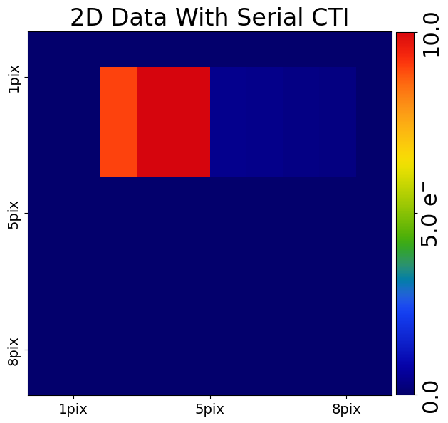
CTI Model (Serial)#
We can do the exact same for serial clocking and CTI.
Because serial clocking is ~x1000 faster than parallel clocking, this means it is subject to a completely different landscape of traps. For this reason, we always define our parallel and serial CTI models separately and it is common for them to have different densities. For illustrative purposes, our serial CTI model has two unique trap species.
The way an electron cloud fills a pixel in the read-out register is different to the main pixels, meaning for serial
clocking and CTI we also define a unique CCDPhase.
serial_trap_0 = ac.TrapInstantCapture(density=2.0, release_timescale=2.0)
serial_trap_1 = ac.TrapInstantCapture(density=4.0, release_timescale=10.0)

serial_ccd = ac.CCDPhase(
    well_fill_power=0.58, well_notch_depth=0.0, full_well_depth=200000.0
)

cti = ac.CTI2D(serial_trap_list=[serial_trap_0, serial_trap_1], serial_ccd=serial_ccd)
We can now add serial CTI to our 2D data by passing it through the 2D clocker.
For our 2d ndarray which has shape (10,8) serial clocking goes left towards entries in the column
pre_cti_data_2d[:, 0]. CTI trails should therefore appear at the right of the pre_cti_data_2d after each
block of 10 electrons.
post_cti_data_2d = clocker_2d.add_cti(
    data=pre_cti_data_2d,
    cti=cti
)

array_2d_plotter = aplt.Array2DPlotter(array=post_cti_data_2d)
array_2d_plotter.figure_2d()
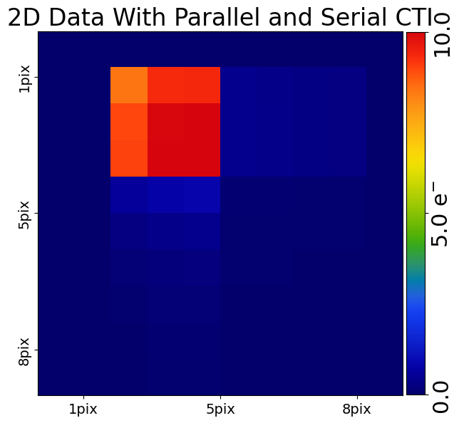
CTI Model (Parallel + Serial)#
We can of course add both parallel and serial via the same arCTIc call.
In this case, parallel CTI is added first, followed by serial CTI, where serial CTI is added on top of the post-cti image produced after parallel clocking. This is the same order of events as occurs on a real CCD.
This means we expect to a small number of electrons trailed into the corner of our post-cti image, which are the parallel CTI trails then trailed during serial clocking.
cti = ac.CTI2D(
    parallel_trap_list=[parallel_trap],
    parallel_ccd=parallel_ccd,
    serial_trap_list=[serial_trap_0, serial_trap_1],
    serial_ccd=serial_ccd,
)

post_cti_data_2d = clocker_2d.add_cti(data=pre_cti_data_2d, cti=cti)

array_2d_plotter = aplt.Array2DPlotter(array=post_cti_data_2d)
array_2d_plotter.figure_2d()
Correcting CTI#
Correcting CTI in 2D is as easy as it was in 1D, by simply calling the clockers remove_cti() method.
corrected_cti_image_2d = clocker_2d.remove_cti(data=post_cti_data_2d, cti=cti)

array_2d_plotter = aplt.Array2DPlotter(array=corrected_cti_image_2d)
array_2d_plotter.figure_2d()

Wrap Up#
We now understand how a CCD works in two dimensions and are able to add and correct CTI to 2D image data.
The remaining question is, if we have data containing CTI which we wish to correct, how do we choose our CTI model? How do we know the density of traps on the CCD? How do electrons fill pixels?
We’ll begin to cover this in the next overview, first explaining how these different properties of the CTI model change the way CTI appears in a dataset; information we will later use to calibrate a CTI model.